Architecture
For contributors — this is the software-engineering view
This page is the code architecture (modules, imports, JIT boundary). If you're an economist evaluating the method, you want the home page instead — the recursive-equilibrium loop and where DEQN sits among projection / time iteration / perturbation, not this import graph.
Three diagrams: the module dependency graph (what imports what), the training cycle sequence (what happens when you call train_from_config), and the ModelSpec contract (what a model author writes vs. what the framework consumes). A fourth section traces tensor shapes through one cycle for the people who think in shapes.
Diagrams are hand-drawn against the actual import graph (extracted via pydeps src/deqn_jax --show-deps) — collapse-at-depth-2 to keep them readable. Regenerate with:
uv run pydeps src/deqn_jax --show-deps --no-output --noshow --max-bacon=4 > /tmp/deps.json
1. Module dependency graph
graph TD
    %% Entry / orchestration
    cli[cli]:::entry
    bench[benchmark]:::entry

    %% Training core
    training[training]:::core

    %% Model authoring
    models[models]:::author
    networks[networks]:::author
    optimizers[optimizers]:::author

    %% Diagnostics
    evaluate[evaluate]:::diag
    irf[irf]:::diag
    plots[plots]:::diag

    %% Shared utilities
    types[types]:::util
    config[config]:::util
    metrics[metrics]:::util

    cli --> training
    cli --> models
    cli --> evaluate
    cli --> irf
    cli --> config
    cli --> optimizers

    bench --> training
    bench --> models

    training --> config
    training --> types
    training --> metrics
    training --> networks
    training --> optimizers
    training --> models

    models --> types
    models -.->|autodiff helper| training

    networks -.->|loss imports| training

    evaluate --> training
    evaluate --> irf
    irf --> training
    irf --> models
    irf --> config

    classDef entry fill:#e1f5fe,stroke:#0288d1,color:#01579b
    classDef core fill:#fff3e0,stroke:#f57c00,color:#e65100
    classDef author fill:#f3e5f5,stroke:#8e24aa,color:#4a148c
    classDef diag fill:#e8f5e9,stroke:#43a047,color:#1b5e20
    classDef util fill:#f5f5f5,stroke:#616161,color:#212121
Reading the graph:
trainingis the hub. Everything that does work goes through it.models,networks,optimizersare author-facing — what you write or extend when porting a new model / new network / new optimizer.evaluate,irf,plotsare diagnostic-only — consume a trained policy + aModelSpec, never touched at training time. (plotshas no inbound deps within the package.)types,config,metricsare leaf utilities.typesdefinesModelSpec/TrainState/Metrics;configis the four Pydantic classes;metricsis the TB / W&B / NullLogger stack.- Two dashed back-edges into
trainingare worth flagging: models -.-> training: only via the autodiff helper (training.autodiff.euler_from_period_return), used by the*_autodiffvariants. Conceptuallytrainingshouldn't be a model dependency, but the autodiff path puts thejax.gradplumbing there. Acceptable given how localized it is.networks -.-> training: a few sequence-network helpers consumetraining.historyfor window construction. Same trade-off.
Ground-truth verification
The diagram above is hand-drawn but validated edge-for-edge against the real import graph: 22 package-level edges in pydeps output, 22 in the mermaid, exact match. Regenerate the diff with:
uv run python scripts/check_module_graph.py
For the full module-level picture (each *.py as a node, clustered by package), here's the auto-generated companion via pydeps:
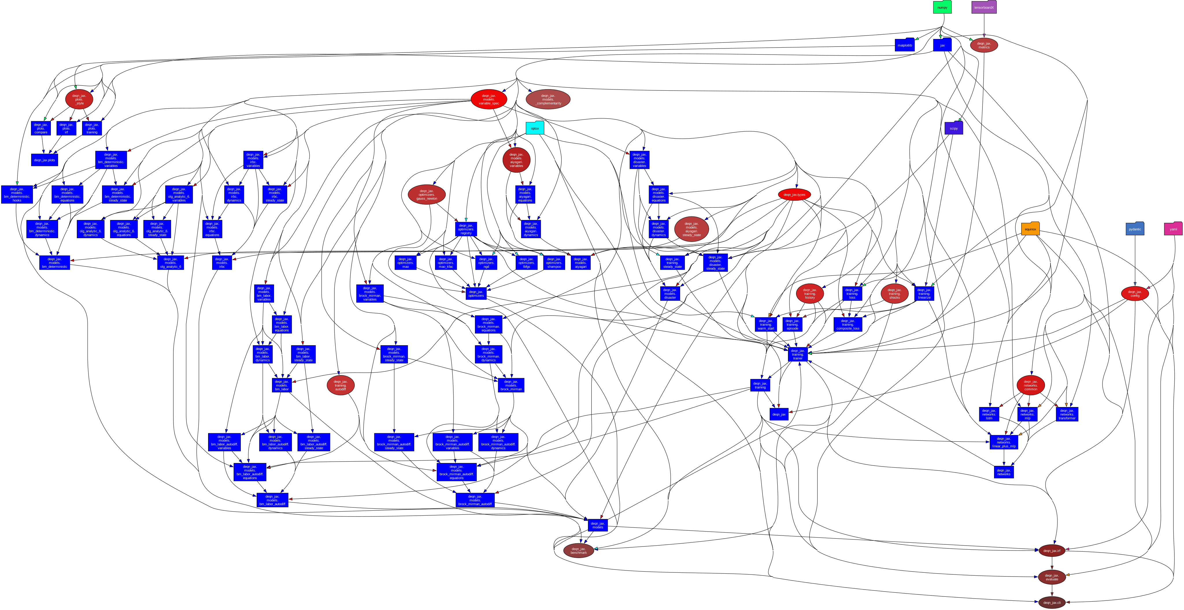
The SVG shows internal package structure too (e.g., the models/<name>/ substructure, individual training/*.py modules, etc.) — useful when "which file in this package?" is the question. The mermaid above is the curated package-level view for getting one's bearings.
2. Training cycle sequence
What happens when you call train_from_config(cfg):
sequenceDiagram
    autonumber
    participant U as User code
    participant TFC as train_from_config
    participant CTS as create_train_state
    participant MTS as make_train_step
    participant CS as cycle_step
    participant RF as rollout_fn
    participant GS as grad_step

    U->>TFC: cfg
    Note over TFC: apply fp64 if requested<br/>composite+opt validation<br/>episode_length=1 / sim_batch / shock_mask checks<br/>load_model + override constants

    TFC->>CTS: model, key, network_config, optimizer_config
    CTS->>CTS: build network (Equinox)<br/>init optimizer<br/>seed history_state if seq policy<br/>sample initial states
    CTS-->>TFC: TrainState, opt, OptimizerKind

    TFC->>MTS: model, opt, kind, ...
    MTS-->>TFC: cycle_step (jit-compiled)

    loop for ep in 0..episodes
        Note over TFC: shock_scale ramp from curriculum
        TFC->>CS: (state, lr_scale, shock_scale)
        CS->>RF: state, shock_scale
        RF->>RF: re-init / ss_reset_frac<br/>run_episode (or _with_history)<br/>=> simulate_step per step
        RF-->>CS: trajectory, final_state, final_history, new_key
        CS->>CS: state._replace(<br/>  episode_state=trajectory[-1],<br/>  history_state=final_history,<br/>  key=new_key)

        loop epochs × minibatches
            Note over CS: shuffle / sorted_within_batch
            CS->>GS: state, minibatch, lr_scale, shock_scale
            GS->>GS: forward + jax.grad on compute_loss<br/>(or jacrev for MAO, or J^T J for GN)
            GS->>GS: opt.update + optax.apply_updates
            GS-->>CS: state', metrics
        end

        CS->>CS: aggregate metrics over sweep
        CS-->>TFC: state, Metrics
        Note over TFC: optional checkpoint, log_every<br/>cycle_hook(model, state, ep)
    end

    TFC-->>U: trained policy_net, history dict
Key things to note:
- One
cycle_step= one rollout + N minibatch grad steps. Everything inside theloopis JIT-compiled; the outer Python loop just dispatches. - Single JIT boundary.
cycle_stepis the single@jax.jitfunction. Validators, checkpointing, logging happen outside JIT. shock_scaleflows through everything — into the rollout (so curriculum andshock_maskapply to state simulation) AND into the loss expectation. Pre-2026-04-24 it only applied to the loss; that bug is now closed.history_statepersists across cycles for sequence policies. For MLP it staysNoneand the path throughcycle_stepis unchanged.
3. The ModelSpec contract
What a model author writes vs. what the framework consumes:
graph LR
    subgraph "Author writes (src/deqn_jax/models/<name>/)"
        VAR[variables.py<br/>SPEC, CONSTANTS,<br/>POLICY_LOWER/UPPER, N_SHOCKS]
        EQ[equations.py<br/>definitions(), equations(),<br/>EQUATION_NAMES]
        DYN[dynamics.py<br/>step]
        SS[steady_state.py<br/>steady_state(),<br/>init_state]
        INIT[__init__.py<br/>MODEL: ModelSpec]
    end

    VAR --> INIT
    EQ --> INIT
    DYN --> INIT
    SS --> INIT

    subgraph "Framework consumes"
        TR[trainer<br/>create_train_state,<br/>make_train_step]
        LOSS[training.loss<br/>compute_loss<br/>compute_residuals]
        EP[training.episode<br/>run_episode,<br/>simulate_step]
        EVAL[evaluate<br/>euler_equation_errors]
        IRFM[irf<br/>run_irf]
    end

    INIT -->|n_states, n_policies, n_shocks| TR
    INIT -->|equations_fn| LOSS
    INIT -->|step_fn| EP
    INIT -->|step_fn, equations_fn| EVAL
    INIT -->|step_fn, equations_fn,<br/>shock_names, definitions_fn| IRFM
    INIT -->|init_state_fn, steady_state_fn| TR
    INIT -->|policy_lower, policy_upper| TR
    INIT -.->|optional: cycle_hook,<br/>state_bounds, definition_bounds,<br/>clip_state_fn| TR
The ModelSpec is a static contract: nothing about it changes during training. The framework reads its fields at training-state construction and at JIT-trace time, then specializes the entire training loop around the model's shapes and equation count. From there the JIT'd cycle step has zero per-step Python dispatch.
4. Tensor shapes through one cycle (for the torchview-minded)
Tracing actual shapes from the start of cycle_step to the end, for a typical config (brock_mirman MLP, batch_size=128, sim_batch=128, episode_length=1, mc_samples=5, n_states=2, n_policies=1, n_shocks=1):
| Step | Object | Shape | Notes |
|---|---|---|---|
| 0 | state.episode_state (in) |
[sim_batch=128, n_states=2] |
Carried from previous cycle |
| 0 | state.params |
pytree of arrays | Equinox MLP, ~10k params |
| 0 | state.history_state |
None (MLP) or [128, H, 2] |
Threaded for sequence policies |
| 1 | init_state_fn redraw (if initialize_each_episode) |
[128, 2] |
Fresh uniform from rect |
| 2 | simulate_step shock |
[128, 1] |
shock_scale * N(0,1), optional shock_mask |
| 2 | policy = policy_net(state) |
[128, 1] |
One forward pass |
| 2 | next_state = step_fn(...) |
[128, 2] |
One step forward |
| 3 | trajectory (lax.scan stack) |
[episode_length=1, 128, 2] |
T-axis prepended |
| 4 | minibatch from trajectory | [batch_size=128, 2] |
Reshape + shuffle |
| 5 | per-shock residuals (vmap) | [mc_samples=5, batch_size=128] per equation |
Inside compute_loss |
| 5 | mean over shocks → per-state residual | [128] per equation |
\(\mathbb{E}_\varepsilon[r]\) for each batch element |
| 5 | square + mean over batch | scalar per equation | MSE |
| 5 | mean over equations | scalar | Loss |
| 6 | grads = jax.grad(loss_fn)(params) |
pytree, same shape as params | |
| 7 | opt.update(grads, opt_state, params) |
pytree of updates | |
| 7 | apply_updates(params, updates) |
new params, same shapes | |
| 8 | state.episode_state (out) |
[128, 2] |
Seeded from trajectory[-1] for next cycle |
For sequence policies (LSTM/Transformer with history_len=H), insert [128, H, 2] for any train_batch and policy-input slot, plus state.history_state is [128, H, 2] instead of None.
For multi-equation models (bm_labor with 2, olg_analytic_6 with 5, disaster with 11), the per-equation residual stack is [mc_samples, batch_size, n_equations] and the mean-over-equations happens at the end before the squared loss.
For Gauss-Hermite quadrature instead of MC, replace mc_samples with n_quadrature_points^n_shocks and the "mean over shocks" becomes a quadrature-weighted sum.
Cross-references
- What is DEQN? — the method itself, in plain economist terms.
- Implementing a model — the author's-side walkthrough of writing the five files in section 3.
- Running experiments — the user's-side walkthrough of the loop in section 2.
- Config reference — every knob that controls section 2's behavior.